With the latest release of Warp 1.5.0, developers now have access to new tile-based programming primitives in Python. Leveraging cuBLASDx and cuFFTDx, these new tools provide developers with efficient matrix multiplication and Fourier transforms in Python kernels for accelerated simulation and scientific computing. In this blog post, we’ll introduce these new features and show how they can be used to optimize your applications. The tile-based programming model available in Warp 1.5.0 is currently in preview – the performance and APIs may change in upcoming versions.
Introduction
Over the past decade, GPU hardware has evolved from a purely SIMT (Single Instruction, Multiple Threads) execution model to one that now relies heavily on cooperative operations for increased efficiency. As Tensor Core math units become a larger part of overall GPU compute, efficiently and productively programming them becomes increasingly important. High-level APIs like BLAS offer abstractions that can target a wide range of high-performance low-level instructions. However, these APIs are often difficult to integrate with user programs and can lose efficiency by, for example, forcing results back to global memory between library calls. Conversely, directly programming Tensor Cores at the C++/CUDA level is complex and demands careful management of data flow between units.
To address these issues, tile-based programming models such as those found in OpenAI Triton and C++ AMP have been developed. Unlike pure SIMT models, tile-based programming allows developers to express operations on tiles that multiple threads can execute cooperatively, enhancing both efficiency and productivity.
With the Warp 1.5.0 release, we extend Warp’s kernel-based programming model to include tile-based operations, aiming to give Warp developers access to the full power of modern GPU hardware. These extensions:
- Provide a programming model that allows developers to smoothly transition from SIMT to tile-based execution.
- Reduce the need for manual indexing, shared memory management, and pointer arithmetic.
- Support auto-differentiation for back-propagation and training.
Additionally, Warp leverages cuBLASDx and cuFFTDx to implement matrix-multiply and Fast Fourier Transform (FFT) tile operations. Combined with Warp’s tile programming model, these NVIDIA device-side math libraries enable seamless fusion of Tensor Core-accelerated GEMM, FFT, and other tile operations within a single kernel, reducing memory I/O and kernel launch overhead, while maximizing arithmetic intensity. With this approach, we can outperform traditional linear algebra or tensor frameworks by a factor of 4x for applications requiring dense linear algebra, such as robot forward dynamics.
Warp tile primitives
The new tile primitives in Warp include construction, load/store, linear algebra, and map/reduce operations in a way that naturally extends the existing kernel-based programming model.
Construction
Tiles may be constructed inside Warp kernels using NumPy-style operations, as shown below:
import warp as wp

@wp.kernel
def compute():


    # construct a 16x16 tile of zeroed 32-bit floats
    a = wp.tile_zeros(m=16, n=16, dtype=wp.float32)


    # construct a 16x16 tile of 16-bit floats initialized to 1.0
    b = wp.tile_ones(m=16, n=16, dtype=wp.float16)
In Warp, tiles are two-dimensional arrays that may contain scalar, vector, matrix, or structured data types as elements. Unlike Warp arrays or PyTorch tensors, where dimensions are dynamic and specified at runtime, the tile dimensions (e.g.,: 16×16 in the above example) must be constants that are known at compile time. Also, unlike SIMT data, which is local to a thread, tile data is stored across an entire CUDA block, either in registers or in shared memory. The full list of tile-construction routines can be found here in the GitHub.
Load/Store
Warp provides explicit load/store operations for tiled data to/from global memory. These operations are performed cooperatively by all threads in the block, ensuring efficient data transfer between global memory and shared or register memory. In the example below, two tiles of data are loaded from global memory, summed together, and the result stored back to global memory. The user doesn’t need to manage shared-memory allocation or storage explicitly:
import warp as wp

@wp.kernel
def compute(A: wp.array2d(dtype=float),
            B: wp.array2d(dtype=float),
            C: wp.array2d(dtype=float)):

    # cooperatively load input tiles
    a = wp.tile_load(A, i=0, j=0, m=16, n=16)
    b = wp.tile_load(B, i=0, j=0, m=16, n=16)

    # compute sum
    c = a + b

    # cooperatively store sum to global memory
    wp.tile_store(C, i=0, j=0, t=c)

A = wp.ones((16,16), dtype=float)
B = wp.ones((16,16), dtype=float)
C = wp.empty((16,16), dtype=float)

wp.launch_tiled(compute, dim=1, inputs=[A, B, C], device="cuda:0", block_dim=64)
In addition to load/store operations, Warp supports atomic operations such as wp.tile_atomic_add(). For the full list of memory operations, please refer to the following documentation.
Matrix multiplication
One of the key benefits of tile-based programming is the ability to perform cooperative matrix multiplication. Warp 1.5.0 introduces a general multiply-accumulate primitive, wp.tile_matmul(), which allows developers to perform cooperative matrix multiplications. Under the hood, this leverages cuBLASDx , which, depending on the element types, matrix size, and data layout, will automatically dispatch the appropriate Tensor Core MMA instruction for best performance.
Let’s walk through an example of using tile-based programming in Warp to perform a matrix multiplication:
import warp as wp

TILE_M = wp.constant(32)
TILE_N = wp.constant(64)
TILE_K = wp.constant(64)

@wp.kernel
def gemm_tiled(A: wp.array2d(dtype=float),
               B: wp.array2d(dtype=float),
               C: wp.array2d(dtype=float)):

    i, j = wp.tid()

    # allocate output tile
    sum = wp.tile_zeros(m=TILE_M, n=TILE_N, dtype=float)
    count = int(K / TILE_K)

    # iterate over inner dimension
    for k in range(count):
        a = wp.tile_load(A, i, k, m=TILE_M, n=TILE_K)
        b = wp.tile_load(B, k, j, m=TILE_K, n=TILE_N)

        # perform gemm + accumulate
        wp.tile_matmul(a, b, sum)

    # store result
    wp.tile_store(C, i, j, sum)


# test with 1024^2 inputs
M, N, K = 1024, 1024, 1024

A = wp.ones((M, K), dtype=float)
B = wp.ones((K, N), dtype=float)
C = wp.empty((M, N), dtype=float)

# launch kernel with 128 threads per-block
wp.launch_tiled(gemm_tiled,
                dim=(int(M//TILE_M), int(N//TILE_N)),
                inputs=[A, B, C],
                block_dim=128)
In this example, we define a kernel gemm_tiled() that performs a tiled matrix multiplication. The kernel loops over 2D slices of data from global memory, loads them into shared memory tiles, performs the matrix multiplication using wp.tile_matmul(), accumulates the result in shared memory, and stores the result back to global memory.
The figure below shows performance of the above GEMM kernel as a percentage of cuBLAS 12.4 on NVIDIA A100 80GB SXM (clocks locked to their maximum) for a range of FP32 matrix sizes. For small problems, we see that performance is competitive with cuBLAS, which may be explained by the fact we have used auto-tuning to find optimal parameters for this small size, and because launch overhead is a more significant portion of the cost. For larger problems, performance is lower since currently tile results are always stored in shared memory. However, even for this simple example, we see approximately 70–80% of cuBLAS performance for larger matrices. Future versions of Warp and cuBLASDx will provide improved performance by keeping the output of GEMMs in registers.

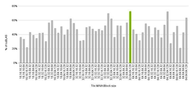
In the figure below, we look at the effect of tile size on overall performance for a single problem size. Overall performance is a function of the tile dimensions, which determines how the problem is decomposed, and the block dimension, which determines how many threads are assigned to each sub-problem. Here, we see that for a M=N=K=1024 problem, the best performance is obtained using tile dimensions of TILE_M=32, TILE_N=64, TILE_K=64, and 128 threads. Warp’s dynamic programming and runtime kernel creation allow users to easily perform auto-tuning of hyperparameters as shown in the example benchmark script.
Please see this reference for a full list of tile linear algebra primitives.
Map/Reduce
Warp 1.5.0 also includes map/reduce primitives, enabling developers to perform reductions and element-wise operations on tiles. These primitives are essential for tasks such as LayerNorm and SoftMax, which require efficient reductions across various quantities.
The example below shows how to compute the sum of all elements in a row of an array using one CUDA block per-row and wp.tile_sum() to perform a cooperative reduction.
import warp as wp

@wp.kernel
def row_sum(input: wp.array2d(dtype=float),
            output: wp.array1d(dtype=float)):

    # obtain our block index
    i = wp.tid()

    # load a row of 256 elements from global memory
    t = wp.tile_load(input[i], i=0, n=256)
    # cooperatively sum elements
    s = wp.tile_sum(t)
    # store sum to output
    wp.tile_store(output, i, s)


a = wp.ones((1024, 256), dtype=float)
b = wp.empty(1024, dtype=float)

wp.launch_tiled(row_sum, dim=[a.shape[0]], inputs=[a, b], block_dim=64)
Warp also supports custom reduction operators, in this example we compute a factorial using the wp.tile_reduce() and wp.mul() builtins, although user-defined @wp.func reduction operators may also be used.
import warp as wp

@wp.kernel
def factorial():
    t = wp.tile_arange(1, 10, dtype=int)
    s = wp.tile_reduce(wp.mul, t)

    # prints "tile(m=1, n=1, storage=register) = [[362880]]"
    print(s)


wp.launch(factorial, dim=[16], inputs=[], block_dim=16)
The full list of map/reduce primitives is available here.

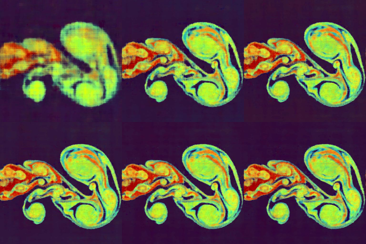
Top: Original image, Bottom: Output of a 4-layer MLP after approximately one minute of training.
Case studies
Fused Neural Networks
Tile-based programming also allows for the efficient implementation of fused multi-layer perceptrons (MLPs). Below we give an example of a fused MLP using tile-based programming in Warp:
import warp as wp


DIM_IN = wp.constant(4)
DIM_HID = wp.constant(32)
DIM_OUT = wp.constant(3)

@wp.kernel
def mlp_fused(weights_0: wp.array2d(dtype=wp.float16),
              weights_1: wp.array2d(dtype=wp.float16),
              loss: wp.array(dtype=float)):


    t = wp.tid()

    # construct simple positional encoding
    x = wp.vec4h(wp.sin(x),
                 wp.cos(x),
                 wp.sin(x*2.0),
                 wp.cos(x*2.0))

    # tile input across block to create feature vectors
    f = wp.tile(x)

    # fully connected layer 0
    w0 = wp.tile_load(weights_0, 0, 0, m=DIM_HID, n=DIM_IN)
    z = wp.tile_map(relu, wp.tile_matmul(w0, f))

    # fully connected layer 1
    w1 = wp.tile_load(weights_1, 0, 0, m=DIM_OUT, n=DIM_HID)
    z = wp.tile_map(relu, wp.tile_matmul(w1, z))

    # loss function
    l = wp.tile_sum(z)

    wp.atomic_add(loss, 0, l)

wp.launch(mlp_fused, dim=(1,), inputs=[weights_0, weights_1, loss], block_dim=128)
In this example, the mlp_fused() kernel evaluates a simple two-layer neural network by loading weights, performing matrix multiplications, applying activation functions using wp.tile_map(), and computing the loss, all within a single kernel.The following image shows an example using this approach to encode an image. Since Warp supports automatic differentiation, we can directly evaluate and train network weights to learn a function that maps from image coordinates (x,y) to pixel color (RGB). The full example is available here.
Signal processing
Warp tile operations integrate cuFFTDx for in-kernel forward and inverse FFTs, providing efficient Fourier-transform operations on tiles of data. Here’s an example of using a tile-based FFT in Warp to compute a convolution using some filter:
import warp as wp

@wp.kernel
def conv_tiled(x: wp.array2d(dtype=wp.vec2d),
  y: wp.array2d(dtype=wp.vec2d),
  z: wp.array2d(dtype=wp.vec2d)):
i, j = wp.tid()

# load signal and filter
a = wp.tile_load(x, i, j, m=TILE_M, n=TILE_N)
f = wp.tile_load(y, i, j, m=TILE_M, n=TILE_N)

# compute Fourier transform of input signal
wp.tile_fft(a)

# compute filter in frequency space
c = wp.tile_map(cplx_prod, a, b)

# convert back to real
wp.tile_ifft(c)
wp.tile_store(z, i, j, c)
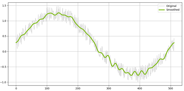
In this example, the conv_tiled() kernel performs the forward FFT of a tile of data (along the last dimension), applies a filter, and then computes the inverse FFT. Under the hood, cuFFTDx is used for the implementation. The full example is available here. The figure below shows the output of applying the filter on a noisy input signal.
Robot forward dynamics
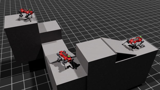
Tile-based programming is also highly beneficial for simulation applications where dense linear algebra is required. In robotic simulation, the Composite Rigid Body Algorithm (CRBA) method is used to compute forward dynamics for articulated mechanisms. In the CRBA method, the following triple-matrix product is required, where the inner matrix M is a block sparse diagonal mass matrix:
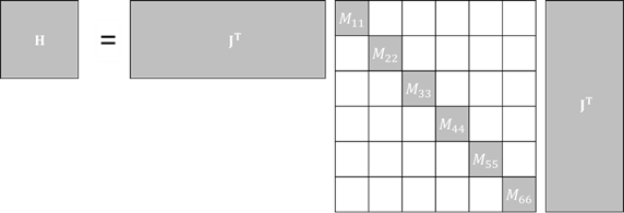
Once constructed, the system matrix is then decomposed using Cholesky decomposition, and solved using forward and back substitution. We can express a batched version of this problem that takes advantage of the sparsity of M using Warp’s tile primitives as follows:
import warp as wp


@wp.kernel
def foward_dynamics(
    J_arr: wp.array3d(dtype=float),
    M_arr: wp.array3d(dtype=float),
    R_arr: wp.array3d(dtype=float),
    H_arr: wp.array3d(dtype=float),
    L_arr: wp.array3d(dtype=float),
):
    batch = wp.tid()

    J = wp.tile_load(J_arr[batch], 0, 0,
  m=wp.static(6 * num_joints), n=num_dofs)
    P = wp.tile_zeros(m=wp.static(6 * num_joints), n=num_dofs, dtype=float)

    # compute P = M*J where M is a 6x6 block diagonal mass matrix
    for i in range(int(num_joints)):


        # 6x6 block matrices are on the diagonal
        M_body = wp.tile_load(M_arr[batch], i, i, m=6, n=6)

        # load a 6xN row from the Jacobian
        J_body = wp.tile_view(J, i * 6, 0, m=6, n=num_dofs)

        # compute weighted row
        P_body = wp.tile_matmul(M_body, J_body)

        # assign to the P slice
        wp.tile_assign(P, i * 6, 0, P_body)

    # compute H = J^T*P
    H = wp.tile_matmul(wp.tile_transpose(J), P)

    # cholesky L L^T = (H + diag(R))
    R = wp.tile_load(R_arr[batch], 0, 0, m=num_dofs, n=1, storage="shared")


    H += wp.tile_diag(R)
    L = wp.tile_cholesky(H)

    wp.tile_store(L_arr[batch], 0, 0, L)

# launch kernel with 64 threads per-robot
wp.launch_tiled(forward_dynamics,
                dim=(num_robots,),
                inputs=[J_arr, M_arr, R_arr, H_arr, L_arr],
                block_dim=64)
In this example, the forward_dynamics() kernel performs the CRBA method by loading tiles of the Jacobian and mass matrices and computing their product to form the system matrix H and its Cholesky factorization. While Torch requires launching a dozen kernels in this particular use case, the Warp implementation requires a single fully fused kernel. This reduces the amount of global memory roundtrips and launch overhead, leading to significantly better performance.
Performance for 1,024 quadruped robots is as follows for the forward dynamics kernel running on an NVIDIA A100 80GB GPU, with all timings in milliseconds (lower is better):
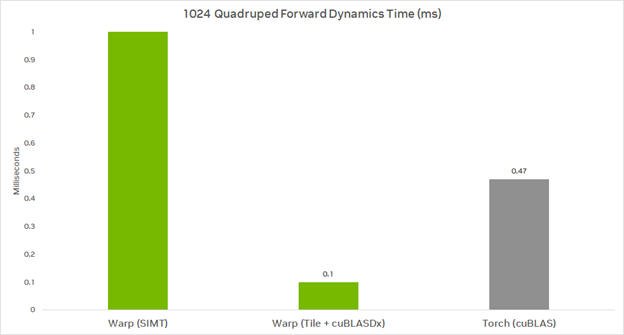
Warp (SIMT) uses an implementation based on its existing SIMT model. Warp (Tile + cuBLASDx) uses the new tile operations. Torch (cuBLAS) uses Torch’s bmm() and cholesky() functions. Note that the Torch implementation is not leveraging the sparsity of M.
The full example is available here, and extensions to expose Cholesky decompositions and back substitution are coming soon.
Future developments
Future versions of Warp and MathDx will include:
- Additional support for row-wise reduction operators
- Tile creation from lambda functions
- Data-type and layout conversions
- Improved performance for GEMM operations
- Additional linear algebra primitives, including various matrix-decomposition algorithms.
Learn more
Tile-based programming in Warp 1.5.0 provides a powerful and flexible approach to GPU programming, enabling developers to achieve significant performance improvements in their applications. By leveraging cuBLASDx and cuFFTDx, Warp 1.5.0 allows seamless fusion of GEMM and FFT operations, reducing memory I/O and kernel-launch overhead.
To get started using Warp’s Tile operations, install Warp in your Python environment using:
To run the fused MLP example, use the following command:
python -m warp.examples.tile.example_mlp.py
To learn more about Warp 1.5.0 and NVIDIA Math device acceleration (Dx) libraries visit the following links:
Acknowledgments
Thanks to Paweł Grabowski, Doris Pan, Neil Lindquist, Jakub Szuppe, Łukasz Ligowski, Sergey Maydanov, and Łukasz Wawrzyniak for their contributions to this post and project.
